Signaler une erreur
Spécialité mathématiques - Travailler sur des sujets du bac
Limites des fonctions, sujet 1
Spécialité mathématiques - Travailler sur des sujets du bac
Limites des fonctions, sujet 1
Imprimer
Spécialité mathématiques - Travailler sur des sujets du bac
Limites des fonctions, sujet 1
Spécialité mathématiques - Travailler sur des sujets du bac
Limites des fonctions, sujet 1
Énoncé
PARTIE A
Soit f la fonction définie sur  par f (x) = x e1−x.
par f (x) = x e1−x.1. Vérifier que pour tout réel x, on a 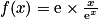 .
.
.2. Déterminer la limite de la fonction f en  .
.
.3. Déterminer la limite de la fonction f en  . Interpréter graphiquement cette limite.
. Interpréter graphiquement cette limite.4. Déterminer la dérivée de la fonction f.
5. Étudier les variations de la fonction f sur , puis dresser le tableau de variations.
, puis dresser le tableau de variations.PARTIE B
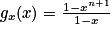
Pour tout entier naturel n non nul, on considère les fonctions gn et hn définies sur par :
gn(x) = 1 + x + x2 + … + xn et hn (x) = 1 + 2x + 3x2 + … + nxn−1.
par :gn(x) = 1 + x + x2 + … + xn et hn (x) = 1 + 2x + 3x2 + … + nxn−1.
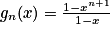
1. Vérifier que pour tout réel x, (1 − x) gn (x) = 1 − xn+1.
On obtient alors, pour tout réel :
:  .
.
On obtient alors, pour tout réel
: .2. Comparer les fonctions hn et  ,
,  étant la dérivée de gn. En déduire que, pour tout réel
  :
: 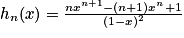 .
.
, étant la dérivée de gn. En déduire que, pour tout réel : .3. Soit Sn = f (1) + f (2) + … + f (n), f étant la fonction définie dans la partie A.
En utilisant les résultats de la partie B, déterminer une expression de Sn puis sa limite quand n tend vers .
.
En utilisant les résultats de la partie B, déterminer une expression de Sn puis sa limite quand n tend vers
.La bonne méthode
PARTIE A
1. Utiliser les règles de calcul de la fonction exponentielle.
2. Limite par produit et composition de fonctions.
3. Utiliser le résultat de la question 1, sachant que 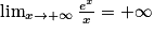 .
.
.4. Dériver un produit de fonctions.
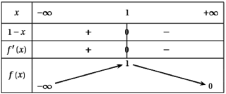
5. Étudier le signe de la dérivée et faire le tableau de variations.
PARTIE B
1. Remplacer gn(x) et développer.
2. Utiliser la dérivée du quotient de deux fonctions. Remarquer une égalité grâce au résultat du 1.
3. Introduire dans Sn la fonction f (x) = x e1−x, puis remarquer l'égalité avec hn(e−1). Enfin, utiliser  .
.
.Corrigé
PARTIE A
1. 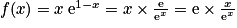 .
.
.2. 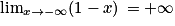 , donc
 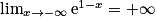 , par composition. Puis, par produit, on obtient que
 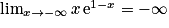 .
.
Donc .
.
, donc , par composition. Puis, par produit, on obtient que .Donc
.3. On sait que  , donc
  . D'où
  .
.
Par conséquent, la courbe représentant la fonction f admet la droite d'équation y = 0 comme asymptote horizontale en .
.
, donc . D'où .Par conséquent, la courbe représentant la fonction f admet la droite d'équation y = 0 comme asymptote horizontale en
.4. f (x) = x e1−x = u (x) ×v (x) avec u (x) = x et v (x) = e1−x. On a  ,
,  et
et 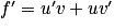 .
.
Donc .
.
, et .Donc
.5. e1−x > 0 donc  est du même signe que 1 − x.
On a donc le tableau de variations suivant :
est du même signe que 1 − x.On a donc le tableau de variations suivant :
 |
PARTIE B
1. (1 − x) gn (x) = (1 − x)(1 + x + x2 + … + xn)
(1 − x) gn(x) = 1 + x + x2 + … + xn − x −x2 −x3 − … − xn+1
(1 − x) gn (x) = 1 −xn+1.
On obtient alors, pour tout réel :
:  .
.
(1 − x) gn(x) = 1 + x + x2 + … + xn − x −x2 −x3 − … − xn+1
(1 − x) gn (x) = 1 −xn+1.
On obtient alors, pour tout réel
: .2. On a  .
.
Or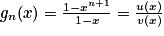 avec u(x) = 1 − xn+1 et v (x) = 1 − x. On a
 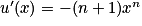 ,
,  et
et  .
.
Donc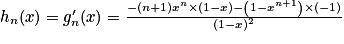
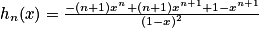

.Or
avec u(x) = 1 − xn+1 et v (x) = 1 − x. On a , et .Donc
3. Sn = 1e1−1 + 2e1−2 + … + ne1−n

Or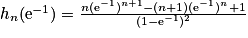
Donc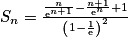 .
.
On a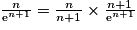 . Or
. Or 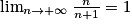 et
et 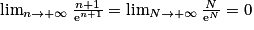 . Donc
 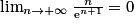 .
.
De même, .
.
On a donc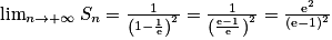 .
.
Or
Donc
.On a
. Or et . Donc .De même,
.On a donc
.Corrigé
PARTIE A
1. .
.2. , donc , par composition. Puis, par produit, on obtient que .
Donc.
, donc , par composition. Puis, par produit, on obtient que .Donc
.3. On sait que , donc . D'où .
Par conséquent, la courbe représentant la fonction f admet la droite d'équation y = 0 comme asymptote horizontale en.
, donc . D'où .Par conséquent, la courbe représentant la fonction f admet la droite d'équation y = 0 comme asymptote horizontale en
.4. f (x) = x e1−x = u (x) ×v (x) avec u (x) = x et v (x) = e1−x. On a , et .
Donc.
, et .Donc
.5. e1−x > 0 donc est du même signe que 1 − x.
On a donc le tableau de variations suivant :
est du même signe que 1 − x.On a donc le tableau de variations suivant :
|
PARTIE B
1. (1 − x) gn (x) = (1 − x)(1 + x + x2 + … + xn)
(1 − x) gn(x) = 1 + x + x2 + … + xn − x −x2 −x3 − … − xn+1
(1 − x) gn (x) = 1 −xn+1.
On obtient alors, pour tout réel : .
(1 − x) gn(x) = 1 + x + x2 + … + xn − x −x2 −x3 − … − xn+1
(1 − x) gn (x) = 1 −xn+1.
On obtient alors, pour tout réel
: .2. On a .
Or avec u(x) = 1 − xn+1 et v (x) = 1 − x. On a , et .
Donc
.Or
avec u(x) = 1 − xn+1 et v (x) = 1 − x. On a , et .Donc
3. Sn = 1e1−1 + 2e1−2 + … + ne1−n
Or
Donc.
On a. Or et . Donc .
De même,.
On a donc.
Or
Donc
.On a
. Or et . Donc .De même,
.On a donc
.
Signaler une erreur
Spécialité mathématiques - Travailler sur des sujets du bac
Limites des fonctions, sujet 1
Spécialité mathématiques - Travailler sur des sujets du bac
Limites des fonctions, sujet 1
Imprimer
Spécialité mathématiques - Travailler sur des sujets du bac
Limites des fonctions, sujet 1
Spécialité mathématiques - Travailler sur des sujets du bac
Limites des fonctions, sujet 1